Page Comparison

The 'ausplotsR' package functions help as pre-processing the AusPlots data extracted with the 'get_ausplots' function into data frames useful for data analysis. For example, the 'species_table' function generates a 'species occurrence by site' matrix (contained in a data frame) from AusPlots raw data (i.e. from point intercept hits in the 'veg.PI' data frame created by the 'get_ausplots' function).

...

An example merging all the data in a 'species_table' data frame ('AP.data.SppbySites.PcC.PFC') and the variables 'bioregion_name', 'longitude', and 'latitude' in the 'site.info' data frame (in the 'AP.data' list) is presented below. The `AP.data' list of data frames contains information for all the currently available AusPlots sites and was previously created in the 'Obtaining AusPlots data: 'get_ausplots' function' Step-by-Step Guide (we use the list created in Example 4). The 'AP.data.SppbySites.PcC.PFC' contains Species by Site data, scored using 'Percent Cover' as scoring metric and .Prejected Foliage Cover as cover type, which was created in the 'Species-Level data: 'species_table' function' Step-by-Step Guide. Before proceeding with the merging, we create a 'site_unique' variable in the 'species_table' data frame to have a common column for merging. The 'site_unique' variable contains a unique id for each site. The required data to create the this variables is present as 'rownames' in the 'species_table' data frame.

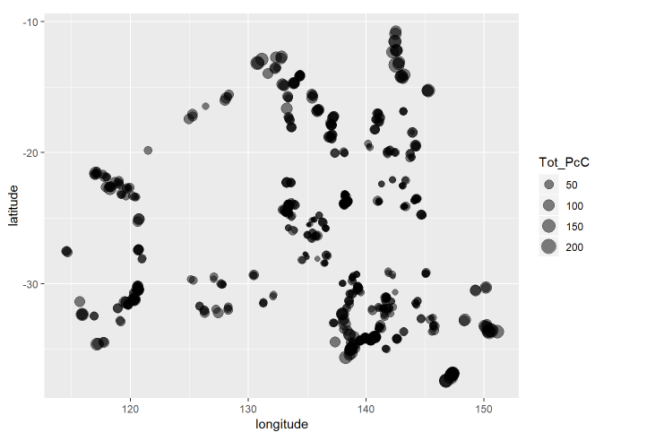
We end the example by creating a new column ('Tot_PcC') containing the Total Percentance Cover from the original values in the 'species_table' data frame and plotting a buble plot representing the Total Percentage Cover in space. To create this plot we use three of the variables we added to the original 'species_table' data frame, 'Tot_PcC', 'longitude', and 'latitude' (the latter two were added in the data frames merge). We use funtions in the 'ggplot2' data visualisation package to generate this plot. More sofisticated graphs of AusPlots data, including graphs of site metrics over a map of Australia, are constructed and displayed in the 'TERN's DSDP 'ECOSYSTEM SURVEILLANCE (AusPlots) TUTORIAL: UNDERSTANDING AND USING THE ‘ausplotsR’ PACKAGE AND AusPlots DATA' tutorial.  

Boxes with grey background contain code snippets, and boxes with white background containt code (text) outputs.

...

# ==================
# Meging data frames
# ==================

# Add the Unique ID ('site_unique') to the Species Occurrence Data Frame
# ----------------------------------------------------------------------
AP.data.SppbySites.PcC.PFC$site_unique = rownames(AP.data.SppbySites.PcC.PFC)
dim(AP.data.SppbySites.PcC.PFC)

...

# Merge Data Frames by Unique ID ('site_unique')
# ----------------------------------------------
# Include all Variables in Species Occurrence Data Frame. To do so use 'names' function,
# and 3 variables in the AP.data$site.info Data Frame (bioregion_name.f, longitude, and latitude)
AP.data.SppbySites.PcC.PFC = merge(AP.data.SppbySites.PcC.PFC, AP.data$site.info, 
                                   by="site_unique")[,c(names(AP.data.SppbySites.PcC.PFC), 
                                                     "bioregion_name", "longitude", "latitude")]
dim(AP.data.SppbySites.PcC.PFC)

...

# Plot
# ----

# Simple version
#plot(AP.data.SppbySites.PcC.PFC$longitude, AP.data.SppbySites.PcC.PFC$latitude, 
#     xlab="Longitude (degrees)", ylab="Latitude (degrees)")

# Compute variable containing the Total Percent Cover per Site ('Tot_PcC')
# '-4' 'cos we have added: 'site_unique', 'bioregion_name', 'logitude', 'latitude'.
AP.data.SppbySites.PcC.PFC$Tot_PcC = rowSums(AP.data.SppbySites.PcC.PFC[,1:(dim(AP.data.SppbySites.PcC.PFC)[2]-4)])
tail(names(AP.data.SppbySites.PcC.PFC))

...

# Plot using functions in 'ggplot2' package
library(ggplot2)
ggplot(AP.data.SppbySites.PcC.PFC, aes(x=longitude, y=latitude)) + geom_point(aes(size=Tot_PcC), alpha=0.5)